Quality issues in AI learning data from various perspectives
Intuitively delivered data quality analysis report
Pebbles Data Clinic provides a baseline quality status of your data, a before and after comparison,
We provide data quality analysis reports, including comparison of two datasets and data life cycle management.
Helps you understand data with scientific analysis and easy-to-understand explanations based on examples and charts.

Pebblous Data Clinic
To all the customers who visited us
Thank you.
“Data Makes AI Makes Data.”
A brave new world is unfolding through the interaction of data and artificial intelligence.
It is a well-known fact that good data makes good artificial intelligence.
The domestic Data Basic Act, which came into effect in 2022, also emphasizes the importance of data quality and seeks to foster the data industry.
Pebblous Data Clinic is a proprietary technology that uses AI and for AI.
We aim to contribute to the data/AI industry by improving the quality of artificial intelligence learning data.

I'll explain in more detail below.
Data quality assessment and improvement for the AI era
Pebblous Diagnostic Report's unique features
Using unique data lens technology
After converting data into a form that can be observed and measured using our self-developed DataLens, we analyze the quality of the data using multifaceted methods such as geometry and statistics. Depending on the customer's needs, we diagnose by applying the optimal DataLens, from ready-made to customized.
Providing customized diagnosis
From traditional Exploratory Data Analysis (EDA) methods to new technologies like DataLens, we provide optimal diagnostics by considering the characteristics of the data and work, as well as the customer's business objectives.


Intuitive and scientific report
Diagnosis at each level provides a variety of charts, diagrams, examples, and explanatory texts to help you understand the multifaceted characteristics of the data more easily and intuitively. The results at each level are summarized and provided in the final results. If necessary, suggestions are made to improve the quality of the dataset.
Identify problems with actual data through diagnostic reports
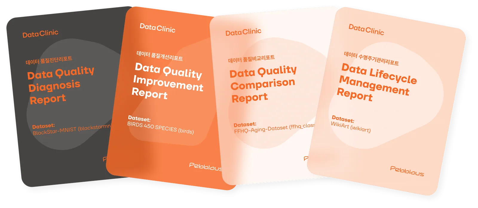
Provided by Data Clinic
Introducing various data quality analysis reports.
Data Quality Diagnostic Report
Comprehensive information on AI learning datasets
Quality diagnosis results and improvement measures
This is a report containing:
Data Quality Improvement Report
Data based on data quality diagnosis results
Quality improvement process such as diet and bulking up
Here is a report explaining the effects.
Data Quality Comparison Report
Before and after quality improvement, learning/test data,
The quality of two datasets, such as similar datasets,
This is a report that provides a detailed comparative evaluation.

Data Lifecycle Management Report
Data quality changes over time.
Market conditions, new regulations, changes in technology, etc.
Considering the current state of the data and the future
Suggest a collection plan.
Structure of a diagnostic report
Step 1
Customer Communication
- Customer's business goals
- Technical Requirements
- Budget and Timeline
Step 2
Comprehensive Evaluation
- Summary of diagnostic results
- Quality Improvement Suggestions
- Diagnostic Level I Summary
- Diagnostic Level II Summary
- Diagnostic Level III Summary
Step 3
Level I Diagnosis
- Measuring Data Integrity
- Missing Value Measurement
- Class Balance Measurement
- Statistical Measurement
Step 4
Level II Diagnosis
- Apply DataLens
- Observing geometric properties
- Observation of distribution properties
Step 5
Level III Diagnosis
- Custom DataLens
- Observing geometric properties
- Observation of distribution properties
Diagnostic Report Guide
all close
Customer Communication
Customer's business goals
Technical Requirements
Budget and Timeline
Comprehensive Evaluation
Summary of diagnostic results
Quality Improvement Suggestions
Level I Diagnostic Summary
Level II Diagnostic Summary
Level III Diagnostic Summary
Level I diagnosis
Measuring Data Integrity
Missing Value Measurement
Class Balance Measurement
Statistical Measurement
Level II diagnosis
Data Lens and Imaging
Observing geometric properties
Observation of distributional properties
Level III diagnosis
Data Lens and Imaging
Observing geometric properties
Observation of distributional properties
Data Diagnostic Report User Guide
We will explain in detail the diagnostic procedures of the data clinic and the composition of the diagnostic report.
Customer Communication
In order to successfully carry out a customer project, we establish the foundation necessary for project execution, such as understanding the customer's business goals, deriving data quality and technical requirements, checking constraints, and domain knowledge, and set diagnostic items and timelines based on this.

1. Customer's business goals
It is a key element that determines the direction of data quality diagnosis. By clearly setting the purpose and goal of the diagnosis, it helps to derive efficient diagnostic methods and finally help the diagnostic results can lead to practical business performance.
2. Technical Requirements
This is related to the tools used in the actual diagnosis (eg algorithm, lens model, etc.), platform, system performance and processing ability. Designed or provided the optimal diagnostic solution for your system infrastructure and technical environment.
3. Budget and Timeline
This is a matter of efficiently distributing project resources such as input budget. Check the diagnostic range and the details of each stage so that all steps can proceed without disruption within the schedule.
Comprehensive Evaluation
From a comprehensive perspective, we synthesize the results of Level I, II, and III diagnostics to evaluate data quality and suggest directions for improvement.


1. Summary of diagnostic results
Considering the comprehensive evaluation opinions on data quality, taking into account the results of the level I, II, III diagnosis and customer communication. It mentions both neutral quality and work -specific quality.
2. Quality Improvement Suggestions
Write a diagnostic report by integrating each analysis result of the diagnostic process introduced earlier. Diagnostic complaints include detailed information on the overall quality, geometric and distribution characteristics of the dataset, the problems and potential values found. In this report, the results of each stage are systematically organized, and the various aspects of the data are widely viewed from the basic characteristics of the data to the advanced characteristics. This clearly understands the quality of the dataset and establishes an efficient data management and utilization strategy. As a result, it contributes to effective big data analysis and artificial intelligence learning.
• Data Diet
Eliminate duplicate/similar data in the dataset and make it lighter while ensuring the performance of the AI model
Utilizing lightweight datasets
Most of the datasets have more duplicate data than you think. Duplicate data is recommended to solve data redundancy because it causes bias in model learning and inefficiency in storage and computational resources. It is also necessary to adjust the amount of data used according to the AI model development process. For example, in the early days, it is more efficient to reduce the size of the data, rather than using the entire dataset for learning. Minimize the use of GPU resources and make it possible to reduce the overall development cycle by enabling fast learning speed.
Class-level optimization
Class -based optimization is the advanced procedure of the data diet. By default, diets at density of the entire data, but furthermore, the data distribution between each class or each class is carefully analyzed to select the data target data. In other words, it emphasizes the core characteristics of each class, while maintaining the distinction between classes. This allows the AI model to recognize each class faster and more accurately and to maximize the performance of the model. It can be applied to the general tasks besides the data diet distinguished.
• Data Bulk-up
Find where data is lacking and generate precision targeting synthetic data suitable for the dataset.

Enhanced class distinction
Data bulk up means adding synthetic data in common terms. However, the Pebellus Data Clinic adds synthetic data with precision burning. In other words, the diagnosis is created through various techniques that find the parts that are relatively lacking in data and create synthetic data. Not only can it improve the distribution quality of the data neutral, but also applicable from a task -specific point of view. For example, bulk -ups relieve the imbalance between classes and help the model to better distinguish each class. It also contributes to strengthening the generalization of the AI model.
• Data Bulk-up
Find where data is lacking and generate precision targeting synthetic data suitable for the dataset.

Improved accessibility and analysis efficiency
It maintains the original data and statistical and distribution characteristics, but it is a virtual data separate from the source data, so it provides a variety of analysis and the possibility of using data without the risk of exposure of sensitive data. By utilizing data replica, it contributes to accelerating data -based decision -making processes by enhancing data accessibility and greatly improving the target range and utility of analysis.
3. Level I Diagnostic Summary
Mentioned the main results for diagnostic items of Measuring data Integrity, Missing value measurement, Class balance measurement, and Statistical measurement.
4. Level II Diagnostic Summary
Among the data lenses that Pebellus have been referred to, we select the characteristics of the target data and the lens that are most suitable for tasks. The characteristics of the data lens, the results of the imaging, the characteristics of the multi -dimensional geometry, the distribution characteristics of the statistical point of view.
5. Level III Diagnostic Summary
Instead of ready -made data lenses, summarize the results of the diagnosis with a special data lens created in consideration of the characteristics and tasks of the target data. Diagnosis is the same as level II.
Level I diagnosis
Level I diagnosis is the most basic EDA stage. At this stage, Measuring data integrity, Missing value measurement, Class balance measurement, Statistical measurement are performed. This stage corresponds to the preliminary work required for the subsequent Level II and III.
 Measuring Data Integrity, Missing Value Measurement,
 Class Balance Measurement, Statistical Measurement
1. Measuring Data Integrity
Data matching evaluation is the first step to ensure the basic quality and reliability of the dataset. In this step, we review the accuracy of metadata, such as the format and size of the dataset, and evaluate the completeness and consistency of the dataset. In particular, if the wrong format or stretch is mixed, it will capture the impact on the dataset, and perform the necessary conformity improvement for the next step.
• Data integrity
In order to ensure the accuracy of all diagnosis in the future, data consistency measures are performed. This measurement focuses on the basic information of the target dataset to check the overall perfection, consistency and accuracy.
Image size
When the image size of the dataset is consistent, it is easy to process and is also efficient for model learning. If the image size is different, the characteristics of the original data can be distorted in the process of adjusting the image to the same size, which can negatively affect the performance of the model. Therefore, it is necessary to make sure that all images have the same resolution. This process is the basis of the quality improvement of the data, reducing the complexity of the data pretreatment process.
Image Channel
The number of channels in the image determines how the image expresses color information. In general, black and white images use 1 channel and color image 3 channels (RGB). For model learning, all images in the dataset must have the same number of channels. If the number of channels is different, an error may occur when the image data is interpreted, which may reduce the consistency and accuracy of the model in the learning process. Even if the number of channels is the same, it may be different, so attention is required. (Yes, RGBA, CMYK)
Label Consistency
The label is a tin information that describes the properties of the image and is used as a reference point for learning the model in the guidance learning. Therefore, the accuracy of the label is an important factor that determines the performance of the model. Since the label error can be directly connected to the error of the learning results, it is very important in the data pretreatment process to make sure it is labeled according to the work features. The criteria for determining the accuracy of the label depend on the tasks, such as sorting, detection, and split work.
2. Missing Value Measurement
Missing tests are the stage of evaluating the integrity of the data. First, identify the context of why the missing value occurs, and then confirm the effect of the side value on the analysis results. After that, we identify the pattern and distribution of the side of the side to determine and propose the appropriate data processing method. This step allows you to understand the characteristics of the dataset more deeply and effectively manage missing information.
• Check for missing values
Missing value measurement is conducted to evaluate the integrity of the data. To do this, we compare the number of data before and after and then after applying the rules of the conclusion processing rules (for example, the side of the side). If there is a difference in the number of data before and after the pre -treatment of the side, there is a high possibility of loss or error in the original dataset.
3. Class Balance Measurement
Class balance measurement is a step to assess the distribution of classes between classes in the dataset. First, identify the frequency of data for each class to identify the imbalance, and if necessary, the data set is balanced by applying the data reassurance or sampling technique. This step can be prevented from the deflection of the model and improved by improving the performance, which can ensure the accuracy and reliability of the analysis results.
• Measuring class balance: number of data per class
Only for datasets with a pre -defined class, the balance measurement by class according to the number of data is performed. To do this, check the statistical information of the training datasets and test datasets for each class.
4. Statistical Measurement
Statistics measurement is a statistically summary of major indicators that show all dataset. The main indicators include the total number of data, the range of data values, and the type of distribution, and also includes basic statistics that are essential for understanding the data. Through this step, it identifies the scope and diversity of the dataset and detects the above value, and identifies the statistical characteristics of the dataset in advance to perform the diagnosis of the future and facilitate interpretation.
• Overall Statistics
Analysis is performed to identify the statistical characteristics of the entire dataset.
Overall average image
The overall average image can be used to gauge the overall trends in color, shape, and pattern of the dataset.
Pixel histogram of the overall average image
You can find out the distribution characteristics of each color channel of the entire average image.
• Statistics by class
Analysis is performed to identify the statistical characteristics of each class dataset.
Average image and average histogram by class
The average image for each class allows you to gauge the class unit trend for the color, form, and pattern of the dataset. Compared to the total average image or other classes, you can also see the specificity of the class.
Level II diagnosis
T0bf08c11
 Pre-learned
 Imaging neural network
 Observation dimension
 Feature Extraction
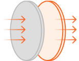
1. Data Lens and Imaging
The selection and imaging of datasens is to analyze the properties of the dataset by selecting a suitable neural network model, a lens. First, select the existing model that accurately reflects the structure of the dataset and can extract the important characteristics properly. Based on this, we measure the geometric properties of the dataset, such as density and distance, and analyze the complexity and diversity of the data. This step allows you to identify the basic structure and pattern of the data, and draw a sketch for establishing subsequent analysis and modeling strategies.
• Select Data Lens
To capture the multi -dimensional characteristics of the data more precisely, select the appropriate data lens and proceed with the data imaging.
Selecting an existing neural network
In order to derive the most efficient analysis results, a large -scale dataset of various domains is used to select a model that best reflects the characteristics of the data among the pre -learned deep learning neural network models. Examples of existing neural networks include Lenet, Resnet-101 (Resnet-101), and Vision Transformer.
Observation dimension
It is the dimensional size of the feature vector printed through the layer of the selected neural network model. This value is the result of the most appropriate optimization of the dimensions that do not lose the complexity and diversity of the dataset. However, the data lens of the level II uses the dimensions of the existing neural network, so it is relatively high for the target dataset.
• Data Imaging
Extract the feature vectors by passing the entire dataset to the existing neural network. At this time, the characteristic vector can accurately reflect the structure of the source data, and then Impeded the values in the manifold in the imaging space and measure the distance and density from the geometric point of view. At this time, the dimensional size of the imaging space is the same as the observation, and the value of each feature vector is one -on -one response to the original data point. Therefore, in order to interpret what the thousands of vector values of hundreds of hundreds of dimensions in the manifold space are meant, the structural step must be essential. In this report, there are two main methods, that is, geometric properties and distribution properties.
2. Observing geometric properties
The geometric property observation is a step of visualizing and observing how far each point in the dataset is in a high -level space. In this case, the two -dimensional PCA visualizes the geometric trend of data that is not revealed in Level I, such as manifold shape in multi -dimensional space and tendency to cluster local clustering. Through this step, you can assess the geometric complexity of the dataset, and clearly grasp the hidden patterns and structural characteristics.
• Macroscopic property observation
Observe the overall structure of the feature vectors and the distribution in the multi -dimensional space. Based on this, you can identify the main geometric characteristics and tendency of the dataset. The optimal observation that calculates the distance and density is still high for visualization, so it is possible to reduce the dimensions by reducing the dimensions using the two -dimensional PCA technique to identify the characteristic vector values at a glance.
Overall data distribution
This is a two -dimensional PCA result to visualize the high -level imaging results obtained with the data lens. In the chart, the origin point (Origin) is a vector value in the imaging space, the average image feature in the imaging space. The higher the diversity of the image, the greater the distance of the average and average image features.
Manifold shape measurement (I) Macroscopic
Observe data imaging results in manifolds in multidimensional space. Horizontal axes are representative classes. The vertical axis is the average of the size of the characteristic vectors in the class, which corresponds to the average of the distance from the origin. The minimum/maximum distance from the origin is displayed together to assess the entire size of the manifold and the specificity of each class. The average image of high diversity data is not similar to any image of the dataset, so it is generally only outside the minimum/maximum section. The data lenses used for level II diagnosis are domain neutral, so the average image is usually present in the minimum/maximum section.
• Observation of local properties
In the topical property measurement, the properties of the individual feature vector values are analyzed in more detail. For example, you can find exception data samples that look like an overtake.
Distance-based similarity measurement
Street -based similarity search results for representative images by class. For example, you can draw 10 closest or farthest data for a given data. This allows you to identify the topical specificity inside the dataset. This helps to identify the overlapping and duplicate images present in the dataset.
Density Measurement (I)
In the multidimensional manifold, which is the result of data imaging, the density is calculated by calculating the distance from each data to the data. The more different data around the specific data, the higher the density, the lower the density. Dense data is likely to be duplicate, and low density data is likely to be an overlapping. Visualization of density is visualized through a two -dimensional PCA, not an observation. The deeper the red color, the more density of the data. In the case of a density measurement by class, a total of 12 classes representing the distribution of density are selected to show the results.
Distance-density measurement
The shape of the multidimensional manifold as a result of data imaging and the density of each data are shown together. The horizontal axis is the distance from the origin of each feature vector, and the vertical axis is the density of the corresponding data. The distance-density chart of a dataset with a good distribution of distance-density measurement results for various data has a single feather shape. Therefore, it is also called a feather chart. Usually, similar/redundant data are located in the dense area at the top of the feather.
Density Measurement (II)
It is similar to density measurement (I), but adds contours so that the distribution of density can be observed with the macroscopic distribution of the data. With the density, the cluster of the macroscopic distribution makes it easier.
3. Observation of distributional properties
Distributable attribute observation is a statistically observed step by visualizing how each point in the dataset is scattered in a high -level space. At this time, histogram, etc., visualizes the macroscopic trend of density, distribution range, coverage, and bias between data points. Through this step, you can understand the overall distribution tendency of the dataset, and specify the various patterns related to this to ensure the essential evidence for data modeling and prediction strategies.
• Observe statistical properties
In order to overall data before the dimension reduction, it analyzes the shape of the entire manifold based on the geometric characteristics of the data and the distance distribution of each data point.
Manifold shape measurement (II) Statistical
The data imaging results are statistically observed in the manifold in the multidimensional space. The horizontal axis represents the frequency of each vector value, the distance from the origin point for each vector value. At this time, the graph marked by the dotted line indicates the flat frequency of the class. This allows you to understand the distribution of a specific class in the manifold. It shows four charts around the reference point. (1) distance from manifold origin, (2) distance from (3) data center at classes by class, (4) distance from data center
Density Measurement (III) Distributional Properties
It shows the distribution of each data density in two charts. First, in the histogram chart, the horizontal axis is density, the vertical axis is the frequency of density. The histogram allows you to understand the overall density distribution of the dataset. In particular, it helps to understand the distribution of the same level as an edge case. The second chart shows the density distribution of representative classes on the box (BOX-WHISKER) chart. Representative classes are arranged in the order of density and can be compared with average density. In the future, if you improve data quality (bulk up/diet), you can also see that the distribution of density is improved.
• Special sample examples
In the entire dataset that does not take into account the class, the highest density samples and the lowest samples are detected each, and each class repeats this task repeatedly. Based on this, you can effectively check the data corresponding to similar or overlapping data and overlapping.
A singular sample from a density perspective
After the quality diagnosis, it shows the unusual samples you need to take a look at the domain knowledge. First of all, it is a peculiar sample of the density point of view. In the entire distribution and the most density for each class, it shows 20 low samples. Dense samples are more likely to correspond to similar/duplicate data and will be subject to data diet later. Low dense samples are unusual samples. Depending on the goal work, bulk -ups may be required to maintain an edge case, remove outlocks, or add data around to increase density.
Level III diagnosis
Custom DataLens & Synthetic-Ready Assessment — Builds a domain-tuned measurement lens paired with a generative lens. Repeats Level II analyses while preparing the foundation for future synthetic-data generation.
 Data Specific
 Imaging neural network
Intrinsic dimension Feature Extraction
 Data Specific
 Generative neural networks
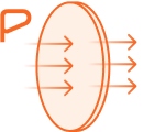
1. Data Lens and Imaging
In addition to selecting the appropriate dataset to capture the complex characteristics of the large dataset, the data imaging is carried out after processing the lens to the dataset. In particular, in the case of level III, it is diagnosed with improvement such as synthetic data creation (data bulk up), redundant data removal (data diet), and reproduction data creation (data replica) for safe data distribution. If you need to improve, you will use your own lens to create synthetic data immediately based on imaging results.
• Data Lens Processing/Selection
To capture the multi -dimensional characteristics of the data more precisely, select the appropriate data lens and proceed with the data imaging.
Observation dimension
Observation is a dimension of the feature vector output through the layer of the selected neural network model. This value is the result of the most appropriate optimization of the dimensions that do not lose the complexity and diversity of the dataset. Unlike level II, the data -specific lens of the level III is processed in accordance with the characteristics of the target dataset, so you can exclude unnecessary elements (for example, backgrounds in images) and capture the target objects required for work. Since a feature vector that does not reflect the inherent characteristics of the data is removed, it can be observed in a much less reduced level of level II. Using the level III's data lens, the feature vectors that reflect the inherent characteristics of the input dataset are the minimum dimension, which is called the intrinsic dimension. In Pevlus, we develop our own and use patented technology to derive the intrinsic dimensions fiercely.
Lens processing type
Select the datalens type type by comprehensively considering the purpose of learning, applying the model, and the characteristics of the data. In particular, the method that best suits the structure and complexity of the dataset is applied.
• Data Imaging
Extract the feature vectors by passing the entire dataset to the existing neural network. At this time, the characteristic vector can accurately reflect the structure of the source data, and then Impeded the values in the manifold in the imaging space and measure the distance and density from the geometric point of view. At this time, the dimensional size of the imaging space is the same as the observation, and the value of each feature vector is one -on -one response to the original data point. Therefore, in order to interpret what the thousands of vector values of hundreds of hundreds of dimensions in the manifold space are meant, the structural step must be essential. In this report, there are two main methods, that is, geometric properties and distribution properties.
2. Observing geometric properties
In this step, we visualize the geometric properties of the dataset obtained through the data custom lens to observe more in -depth. In Level II, which uses existing neural networks, we examine more precisely interrelationship between data points, spatial placements, and complex structures in datasets. Through this step, you can establish a more advanced data analysis strategy by identifying geometric complexity and patterns due to the inherent attributes of data.
• Macroscopic property observation
Observe the overall structure of the feature vectors and the distribution in the multi -dimensional space. Based on this, you can identify the main geometric characteristics and tendency of the dataset. The optimal observation that calculates the distance and density is still high for visualization, so it is possible to reduce the dimensions by reducing the dimensions using the two -dimensional PCA technique to identify the characteristic vector values at a glance.
Overall data distribution
This is a two -dimensional PCA result to visualize the high -level imaging results obtained with the data lens. In the chart, the origin point (Origin) is a vector value in the imaging space, the average image feature in the imaging space. The higher the diversity of the image, the greater the distance of the average and average image features.
Manifold shape measurement (I) Macroscopic
Observe data imaging results in manifolds in multidimensional space. Horizontal axes are representative classes. The vertical axis is the average of the size of the characteristic vectors in the class, which corresponds to the average of the distance from the origin. The minimum/maximum distance from the origin is displayed together to assess the entire size of the manifold and the specificity of each class. The average image of high diversity data is not similar to any image of the dataset, so it is generally only outside the minimum/maximum section. The data lenses used for level II diagnosis are domain neutral, so the average image is usually present in the minimum/maximum section.
• Observation of local properties
In the topical property measurement, the properties of the individual feature vector values are analyzed in more detail. For example, you can find exception data samples that look like an overtake.
Distance-based similarity measurement
Street -based similarity search results for representative images by class. For example, you can draw 10 closest or farthest data for a given data. This allows you to identify the topical specificity inside the dataset. This helps to identify the overlapping and duplicate images present in the dataset.
Density Measurement (I)
In the multidimensional manifold, which is the result of data imaging, the density is calculated by calculating the distance from each data to the data. The more different data around the specific data, the higher the density, the lower the density. Dense data is likely to be duplicate, and low density data is likely to be an overlapping. Visualization of density is visualized through a two -dimensional PCA, not an observation. The deeper the red color, the more density of the data. In the case of a density measurement by class, a total of 12 classes representing the distribution of density are selected to show the results.
Distance-density measurement
The shape of the multidimensional manifold as a result of data imaging and the density of each data are shown together. The horizontal axis is the distance from the origin of each feature vector, and the vertical axis is the density of the corresponding data. The distance-density chart of a dataset with a good distribution of distance-density measurement results for various data has a single feather shape. Therefore, it is also called a feather chart. Usually, similar/redundant data are located in the dense area at the top of the feather.
Density Measurement (II)
It is similar to density measurement (I), but adds contours so that the distribution of density can be observed with the macroscopic distribution of the data. With the density, the cluster of the macroscopic distribution makes it easier.
3. Observation of distributional properties
In this step, we visualize the distribution properties of the dataset obtained through the data custom lens to observe more in -depth. Similarly, we will examine more precisely the density, dispersion, and distributed characteristics between data points that are difficult to identify in Level II. Through this step, you can accurately recognize the distribution complexity and diversity of the dataset to establish a more sophisticated data modeling strategy.
• Observe statistical properties
In order to overall data before the dimension reduction, it analyzes the shape of the entire manifold based on the geometric characteristics of the data and the distance distribution of each data point.
Manifold shape measurement (II) Statistical
The data imaging results are statistically observed in the manifold in the multidimensional space. The horizontal axis represents the frequency of each vector value, the distance from the origin point for each vector value. At this time, the graph marked by the dotted line indicates the flat frequency of the class. This allows you to understand the distribution of a specific class in the manifold. It shows four charts around the reference point. (1) distance from manifold origin, (2) distance from (3) data center at classes by class, (4) distance from data center
Density Measurement (III) Distributional Properties
It shows the distribution of each data density in two charts. First, in the histogram chart, the horizontal axis is density, the vertical axis is the frequency of density. The histogram allows you to understand the overall density distribution of the dataset. In particular, it helps to understand the distribution of the same level as an edge case. The second chart shows the density distribution of representative classes on the box (BOX-WHISKER) chart. Representative classes are arranged in the order of density and can be compared with average density. In the future, if you improve data quality (bulk up/diet), you can also see that the distribution of density is improved.
• Special sample examples
In the entire dataset that does not take into account the class, the highest density samples and the lowest samples are detected each, and each class repeats this task repeatedly. Based on this, you can effectively check the data corresponding to similar or overlapping data and overlapping.
A singular sample from a density perspective
After the quality diagnosis, it shows the unusual samples you need to take a look at the domain knowledge. First of all, it is a peculiar sample of the density point of view. In the entire distribution and the most density for each class, it shows 20 low samples. Dense samples are more likely to correspond to similar/duplicate data and will be subject to data diet later. Low dense samples are unusual samples. Depending on the goal work, bulk -ups may be required to maintain an edge case, remove outlocks, or add data around to increase density.